
One – Point estimation reflects one value per activity. It is based on expert judgement, experience, expert opinion or historical information. Fear of padding is always a major concern with one-point estimation. Also, it does not reflect risk or uncertainty associated to schedule or cost estimation. Therefore, Three-point (3) estimation is preferred for activity duration (schedule) and cost estimation. Three-point (3) estimation ‘PERT’ uses pessimistic (P), most likely (M) and optimistic (O) for estimation. PERT is also called as ‘Weighted Average’ (not just an average). It is calculated by a formula:
PERT =(P+4M+O)/6
PERT provides the basis to calculate Activity Standard Deviation, Activity Variance and Project Variance and Project Standard Deviation.
Activity Standard Deviation = (P-O)/6
Activity Variance = ((P-O)/6)^2
Project Variance = ∑((P-O)/6)^2
Project Standard Deviation = √(Project ) Variance
Let’s take an example of a ‘Pressure Vessel Design and Commissioning Project’ to enlighten PERT Analysis. Assume that there are four phases in a project, i.e. design, fabrication, testing and commissioning. The client has given 70 days to complete the project. Project planning team assess the duration of project phases as given below:
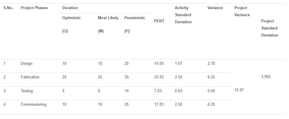
According to calculations, project will be completed in 66.60 ~67 days. It portrays the project will be completed before the deadline. Wow, sounds great! Is it the real story? Would it be the only information to rely on? The answer is no, project completion depicts only the one façade of the situation. Perhaps one requires more calculations to have a complete picture of a scenario. Therefore, it is required to first find out the probability to meet the deadline on the basis of planning. Probability to finish project within a deadline of 70 days can be found by ‘Z’ (Standard Normal Equation).
According to calculations, project will be completed in 66.60 ~67 days. It portrays the project will be completed before the deadline. Wow sounds great! Is it the real story? Would it be the only information to rely on? Answer is no, project completion depicts only the one façade of the situation. Perhaps one requires more calculations to have a complete picture of a scenario. Therefore it is required to first find out the probability to meet the deadline on the basis of planning. Probability to finish project on deadline of 70 days can be found by ‘Z’ (Standard Normal Equation). Where ‘Z’ is the number of standard deviations the due date or target date lies from the mean or expected date. Project Standard Deviation is already calculated 3.995~4 days. So in order to calculate the probability, the standard normal equation can be applied as follows:
Z = (Due Date-Expected Date of Completion)/σp
= (70 days – 67 days)/4 days = 0.75
Now referring to ‘Normal Curve Area Table’* to find out the area under the normal curve. From the table, the probability is found 0.77337. Thus, there is a 77.337 % chance that ‘Pressure Vessel Design and Commissioning Project’ can be completed in 70 days or less. What if to know the 99 % probability to meet the deadline? 99% chance to complete the project can be calculated by formula as given below:
Due Date = Expected Due Date+Z* σP
= 67 + 2.33** X 4 = 67 + 9.32
= 76.32 ~ 76 Days
PERT Analysis reveals that there is a requirement to compress the schedule at least 6 days to meet the client’s deadline.
While discussing the topic, ‘An Approach to Perform Project PERT Analysis Manually’, one of the Senior Risk expert put an awe-inspiring scenario before me and asked me to give a solution to the scenario as described below:
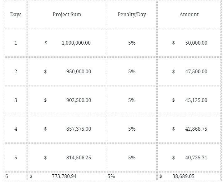
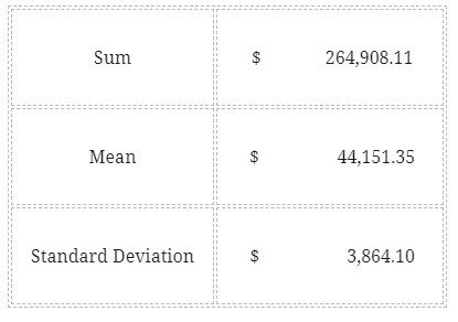
“Now assume that the Client reduces that project sum by 5% for every day that the project is delivered late: Calculate the (average) expected claim that the Client will have if the project is not shortened by 6 days. And for the advanced: What is the standard deviation of the claim. Now you can say how much the reduction in project time is allowed to cost and still be cost effective.”
His question really provoked me to think out of the box. The solution I proposed is given below:
“Your questions are a bit tricky and require some assumptions. First award or penalty is agreed before commencing the project. Either CPIF/CPAF or FPIF contract is usually workable depending upon the prevailing circumstances. Now come to your questions. As I conceived outcomes may be calculated by assuming some values. Assume that project sum is M 1 USD ($ 1,000,000). If the penalty is 5%/day on project sum, then it would be like…..”
I just rolled the ball again in his court, wow :). He replied as:
“Your sums are correct but the answer is much simpler. The six days are worth 6 x $50k = $300k. If it costs you more than $300k to avoid the 6 days delay (and it will not become more!), do not change and incur the $300k claim (Liquidated damage, or LD). If you can correct (e.g. avoid the 6 days overrun) at a cost of less than $300k, say $200k, then you have “increased” the profit on the project from $700k to $800k. Do realize that when you discovered that you “certainly” would have a six (6) day schedule overrun, your project had decreased in value from $1000k to $700k.
The standard deviation comes in when the 6 days overrun are uncertain, or when the corrective action of $200k is uncertain or whether the corrective action has a 100% chance of avoiding the schedule overrun. This will make it all very complex without giving extra “message” to your management. That message, in fact is: Either accept the loss of $300k because correction costs more, or apply the corrective action and improve the position that has already happened, e.g. the drop in value from $1000k to $700k.
Of course it all assumes that the Client does not become so angry with the 6 days overrun that he will not buy from you again. But then the cost of the 6 day overrun must also include the lost profit on the next project. And then a corrective action of say $400k may still be good economics for your company and for the project. “
Another Risk savvy presented the solution differently as:
“As a general comment, if your project duration forecast distribution looks like a Normal distribution, it is very likely that you didn’t include (enough) relationships between tasks. Also, you should review if you took into account the true risks that would cause the project to take a lot more time than expected. A more typical forecast distribution would look right-skewed, i.e. have a long ‘right tail’.
Aside from this, you raised an interesting question. The use of the standard deviation as a measure of risk is really mostly useful when your distribution is (approximately) Normally distributed. When this is not the case, the interpretation (and calculations with) a standard deviation become a lot harder. So, in your case, assuming that the total duration of the project indeed follows a Normal distribution, there would be about a 77% probability that you will meet the deadline and therefore a 23% probability of not meeting it. Given that you don’t make the deadline, your expected value is 72.32 days (you can easily see then we specifying a Normal distribution with mean = 67, StDev = 4 and Lower Truncation = 70). Your expected value therefore is 23% * 2.32 * $50,000 = $27K (i.e. this is the expected claim the client will have). Your expected value given that you do have an overrun is 2.32 * $50,000 = $116K (i.e. this is the expected value, conditional that you do have an overrun). I would recommend against using a standard deviation in this case, since this really doesn’t give a lot of insight. What you could do instead is show the actual distribution of claims (preferred option), or alternatively calculate a P10 and P90, since percentiles are easier to interpret and have the same interpretation, independent what distribution you are considering.”